

Perform data wrangling using python to create useful datasets for visualising property transactions! This is in continuation of the URA API series.
Below contains data wrangling python scripts to create datasets for useful visualisations later
- 1. Import the required libraries
- 2. Invoke the necessary parameters to work with the transaction file
- 3. Read the csv file
- 4. Filter for property tranasctions for EC & Private Condos. Get the average area sqft of each transaction record
- 5. Aggregrate the transactions by Project & No. of Bedrooms
- 6. Convert x y coordinates to lat long coordinates
- 6. Filter for visualisation dataset for 3 bedder condos
- 7. Categorise the transactions to fall under 25th, 50th, 70th percentiles to visualise it in bubble plots
- 8. Save the df_merged and three_bedder_df to csv files
1. Import the required libraries
import pandas as pd
import csv
import json
import numpy as np
import re
2. Invoke the necessary parameters to work with the transaction file
# Enter the refperiod of your transaction file
refperiod = "23q3"

# Extract the year and quarter using regular expressions
match = re.match(r'(\d{2})q(\d)', refperiod)

if match:
    year = match.group(1)
    quarter = int(match.group(2))

    # Calculate the start month
    start_month = str((quarter - 1) * 3 + 1).zfill(2)

    # Calculate the end month
    end_month = str(quarter * 3).zfill(2)

    # Combine the year and month to get the desired format
    startMonthID = start_month + year
    endMonthID = end_month + year

    print("Start Month:", startMonthID)
    print("End Month:", endMonthID)
else:
    print("Invalid refperiod format.")
Example output: Start Month: 0723 End Month: 0923
3. Read the csv file
df = pd.read_csv(f'transaction_resi_converted_raw_csv_{refperiod}.csv', converters = {'leaseDate': str, 'noOfBedRoom': str})
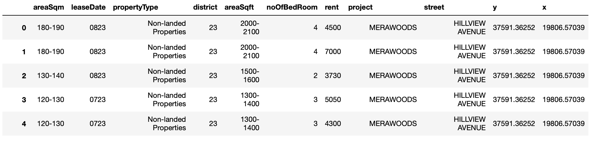
4. Filter for property tranasctions for EC & Private Condos. Get the average area sqft of each transaction record
df = df[df.propertyType.isin(["Non-landed Properties", "Executive Condominium"])]
df = df[df.noOfBedRoom.isin(["1","2","3","4","5"])]
df['areaSqft'] = np.where(df['areaSqft'] == '>3000', '3000-3000', df['areaSqft'])
df[['areaSqft_lower', 'areaSqft_higher']] = df['areaSqft'].str.split('-', expand=True)
df = df.astype({"areaSqft_lower":"int","areaSqft_higher":"int"})
col = df.loc[: , "areaSqft_lower":"areaSqft_higher"]
df['mean_areaSqft'] = col.mean(axis=1)
df
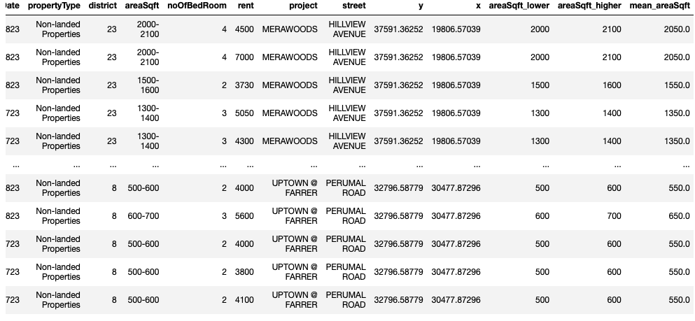
5. Aggregrate the transactions by Project & No. of Bedrooms
df = df.groupby(['project', 'noOfBedRoom','propertyType']).mean().reset_index()
df = df.replace(to_replace="Non-landed Properties",
           value="Private Condominium")
df = df.astype({"mean_areaSqft":"str"})
df.dtypes
df['mean_areaSqft'] = np.where(df['mean_areaSqft'] == '3000.0', '>3000', df['mean_areaSqft'])
df = df.drop(['areaSqft_lower', 'areaSqft_higher'], axis=1)
df
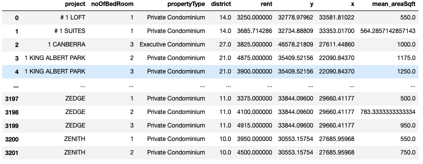
6. Convert x y coordinates to lat long coordinates
I make use of a open source python script to do so. You may check out the script over here: github repository
# generate a separate csv as input file for SVY21.py script
# to convert x y coordinates to lat long coordinates
x_y_coord_df = df.drop(['project', 'noOfBedRoom', 'district', 'rent', 'mean_areaSqft'], axis=1)
x_y_coord_df.to_csv(f'x_y_coord_df_{refperiod}.csv', na_rep='N/A', quoting=csv.QUOTE_NONE, index=False)
# run python SVY21.py x_y_coord_df_23q3.csv output_x_y_coord_df_23q3.csv
# output file will have lat & long coordinates
lat_long_df = pd.read_csv(f'output_x_y_coord_df_{refperiod}.csv')
# simple joining using index
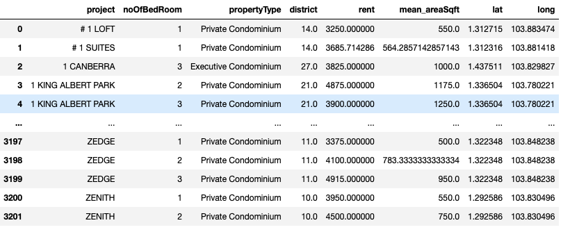
df_merged = df.join(lat_long_df)
df_merged = df_merged.drop(['y', 'x'], axis=1)
df_merged.rename(columns= {'Y': 'lat' , 'X': 'long'}, inplace = True)
df_merged
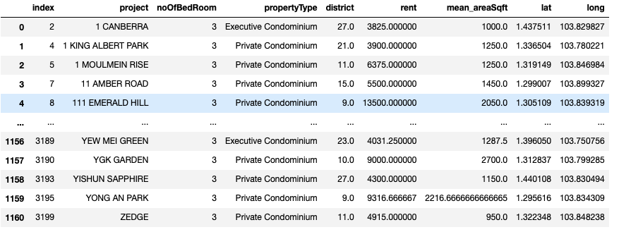
6. Filter for visualisation dataset for 3 bedder condos
three_bedder_df  = df_merged[df.noOfBedRoom.isin(["3"])].reset_index()
three_bedder_df
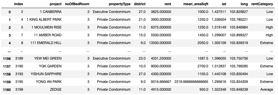
7. Categorise the transactions to fall under 25th, 50th, 70th percentiles to visualise it in bubble plots
A transaction rental record would be tagged as ‘Low’, Average’, High’, ‘Extreme’ according to the percentile category it falls under. These 4 categories would be represented with different bubble colours in the interactive map later.
three_bedder_df_25th = three_bedder_df.groupby(['noOfBedRoom']).quantile(.25).rename(columns={"rent": "25th_rental"})
three_bedder_df_50th = three_bedder_df.groupby(['noOfBedRoom']).quantile(.50).rename(columns={"rent": "50th_rental"})
three_bedder_df_75th = three_bedder_df.groupby(['noOfBedRoom']).quantile(.75).rename(columns={"rent": "75th_rental"})

def conditions(s):
    if s['rent'] < three_bedder_df_25th['25th_rental'].iloc[0] :
        val = 0
    elif s['rent'] < three_bedder_df_50th['50th_rental'].iloc[0] :
        val = 1
    elif s['rent'] < three_bedder_df_75th['75th_rental'].iloc[0] :
        val = 2
    else:
        val = 3
    return val

three_bedder_df['rentCategory'] = three_bedder_df.apply(conditions, axis=1)
three_bedder_df = three_bedder_df.replace({'rentCategory': {0:'Low', 1:'Average', 2:'High', 3:'Extreme'}})
three_bedder_df
8. Save the df_merged and three_bedder_df to csv files
# export df_merged into csv
df_merged.to_csv(f'transactions_resi_project_bedroom_index_{refperiod}.csv', na_rep='N/A', quoting=csv.QUOTE_NONE, index=False)
# export three_bedder_df into csv
three_bedder_df.to_csv(f'transactions_three_bedder_{refperiod}.csv', na_rep='N/A', quoting=csv.QUOTE_NONE, index=False)
We have now prepared 2 datasets for useful visualisations later.